R Variables and Constants (Chapter 1 Episode 3)

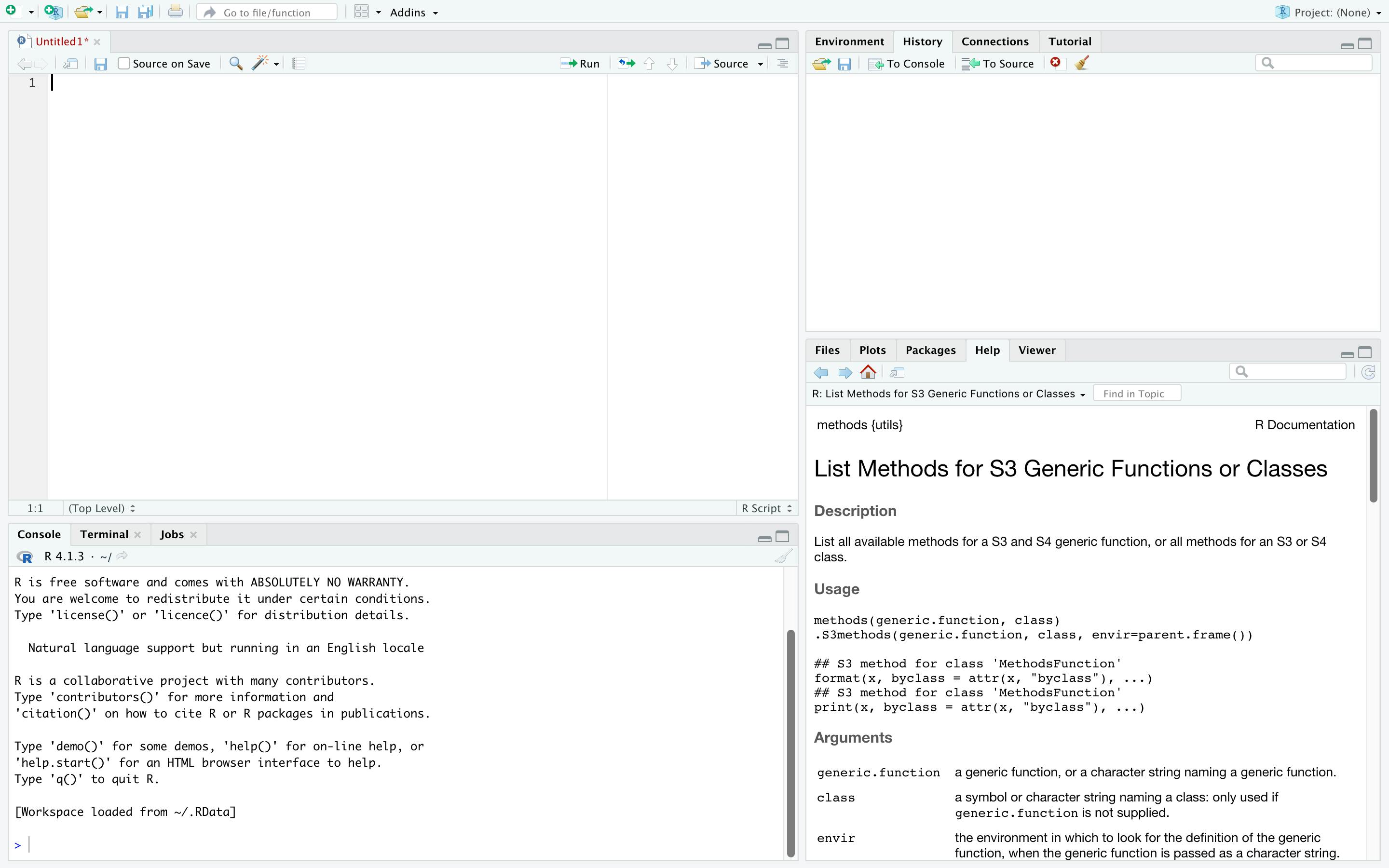
In this lesson, we are going to talk about the data types we have in R and get you ready for your data science career. After installing the software, go ahead and open up the R studiodata type

To create a new workspace , go to file > New file > R script

Variables are used for storage of data, whose value can change based on our need. Each R variable is given a unique name, and this is called the identifier. Here are the rules that govern the writing of identifiers in R:

• An identifier can have a combination of letters, digits, period (.) and underscore (_).

• The identifier must begin with either a letter or a period. If the identifier begins with a period, then it cannot be followed by a digit.

• The reserved R keywords cannot be used as identifiers.

Here are examples of valid identifiers in R: name, Sum, .okay.with.dot, this_is_acceptad, Position5.

Variable Assignment

The leftward, rightward and equal operators can be used for assigning values to variables. To print the value of the variable, you can use the “print()” or the “cat()” function. The “cat()” function will combine the multiple items so as to get a continuous output. Consider the example given below:

The equal operator for variable assignment

var.1 = c(5,6,7,8)

The leftward operator for assignment:

var.2 <- c("learn programming in","R")

The rightward operator for assignment

c(TRUE,1) -> var.3

Constants in R

A variable can store values ranging from:

• logical

• numeric

• integer

• complex

• character

logical Constants

The logical data type is also known as boolean as it values are either TRUE or FALSE

value1 < - TRUE
 print(value1)
print(class(value1))

output

[1] TRUE
[1] "logical"

Alternatively, you can also assign the value of TRUE to be T and FALSE to be F.

numeric data type

The numeric data type refers to numbers with or without decimal points.

number < - 12
print(number)
print(class(number))

count < -  16.67
print(count)
print(class(count))

output

[1] 12
[1] "integer"

[1] 16.67
[1] "numeric"

integer Constants

R has a way of recognising integer value and this is by adding L to it. Integer values are also numeric values in space if numeric data type. These constants ends with L.

x <- 15L
print(x)
print(class(x))

output [1] 15 [1] "integer"

We can use integer as hexadecimal.

 x <- 0x17L
print(x)

output

[1] 23

complex Constants

A complex number contains a real number and an imaginary variable (denoted by i).

 y <- 4.2e-1i
print(y)
print(class(y)

output

[1] 0+0.42i
[1] "complex"

character Constants

String data type can be numeric, alphabets or alphanumeric.

message <- "Hello World"
print(message)

output

[1] "Hello World"

Built-in R constants

R programming provides some predefined constants that can be directly used in our program.

# print list of uppercase letters
print(LETTERS)

# print list of lowercase letters
print(letters)

#print the months of the year
print(month.name)

# print 3 letters abbreviation of English months
print(month.abb)

# print numerical value of constant pi
print(pi)

> print(LETTERS)
 [1] "A" "B" "C" "D" "E" "F" "G" "H" "I" "J" "K" "L" "M" "N" "O" "P" "Q" "R" "S" "T" "U" "V" "W" "X" "Y" "Z"
> print(letters)
 [1] "a" "b" "c" "d" "e" "f" "g" "h" "i" "j" "k" "l" "m" "n" "o" "p" "q" "r" "s" "t" "u" "v" "w" "x" "y" "z"
> print(month.name)
 [1] "January"   "February"  "March"     "April"     "May"       "June"      "July"      "August"    "September" "October"   "November"  "December" 
> print(month.abb)
 [1] "Jan" "Feb" "Mar" "Apr" "May" "Jun" "Jul" "Aug" "Sep" "Oct" "Nov" "Dec"
> print(pi)
[1] 3.141593

In the examples above,

LETTERS - displays a list of the English Alphabets in upper case

letters - displays a list of the English Alphabets in lower case

month.name - displays a list of all the months of the year

month.abb - displays a list of all the months of the year abbreviated

pi - displays the maths pi constant value

Finding Variables

To find all the variables that are contained in your workspace, you can use the ls() function.

ls()

output

[1] "addNum"        "age"           "c"             "column"        "count"         "greeting"     
 [7] "greetings"     "info"          "items"         "listNames"     "matri"         "matri2"       
[13] "message"       "mult"          "mult2"         "multNum"       "mylist"        "myMatrix"     
[19] "name"          "num1"          "num2"          "number"        "numbers"       "print.Student"
[25] "r"             "result"        "row"           "s1"            "s2"            "s3"           
[31] "senum"         "seq2"          "seq4"          "student"       "studentInfo"   "students"     
[37] "value"         "value1"        "value2"        "vector1"       "vector2"       "vector3"      
[43] "vectorA"       "vectorB"       "x"             "y"

The command can be used as follows with patterns: To see all the variables whose identifiers, begin with pattern "num"

ls(pattern='num')

output

[1] "num1"    "num2"    "number"  "numbers" "senum"

Deleting Variables

To remove a variable, we can use the rm() function. Suppose we need to delete a variable with the name “num2”. We only have to invoke the rm() function and pass the name of the variable to it as the argument. This is demonstrated below:

rm(num2)

If I try to get the value assigned to num2 after running the above, I get an error:

> num2
Error: object 'num2' not found

To delete all the variables in the workspace.

rm(list=ls())

Getting User Input

To allow users to enter the input data, you can call the readline() function. This function reads data from the user and stores it in a variable. We can then access the data through that variable. Let us create an example that demonstrates how this can be done:

#asks the user to enter their name
name <- readline(prompt="Enter your name: ")

#asks the user to enter their age
age <- readline(prompt="Enter your age: ")